Chapter 5 – Interactions

Feynman diagrams

Richard Feynman created diagrams showing particle interactions. They have time along one axis and show particles interacting at vertices along the time line. Here is a simple diagram:

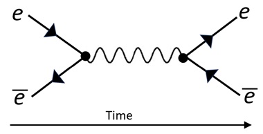
This starts with an electron and a positron (that is an anti-electron which is labeled as a with a bar over it). By convention, anti-particles have arrows going backwards.

• At the first vertex, the particles are annihilated and a photon is generated. Photons are shown with wavy lines.
• At the second vertex the photon changes to an electron and positron.

Note: The resulting particles did not exist before the interaction and are spontaneously created

Diagrams can be rotated

A rotated diagram shows an equally valid interaction. The new direction of the arrows can cause particles and anti-particles to be swapped.

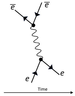
This rotated version of the last diagram describes a different interaction between an electron and a positron.

• A positron changes to a positron and a photon
• An electron absorbs the photon to give a new electron

More than just pictures

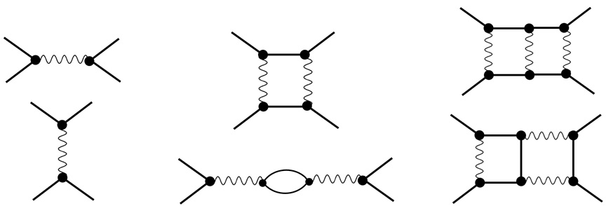
Feynman diagrams give a formal way of calculating the probability of an outcome by considering the infinite variations that achieve a result and adding them up!

How can an infinite number of variations be added up?

Infinite series can be summed if the values go down rapidly. For exaample:

1 + 1/2 + 1/4 + 1/8 + 1/16 + ….. = 2.0

Each extra level of complexity in the Feynman diagram reduces contribution by the fine structure constant (about 1/137). To see how quickly this converged consider adding an infinite number of terms:

1 + 1/137 + 1/137² + 1/137³ + …. = 1.00735294

If we just stop after two terms we get the answer correct to 6 decimal places:

1 + 1/137 + 1/137² = 1.00735255

This allows the probabilities of different interactions to be calculated without really having to look at all infinite number of variations